Ever wonder how a computer "sees" the world? It doesn't perceive a lush landscape or a busy city street like we do. Instead, it starts by playing a game of connect-the-dots, and the first step is figuring out where the dots even are. This is the magic of edge detection.

It's a core technique in image processing that pinpoints the boundaries of objects by looking for sudden, dramatic shifts in brightness. Think of it as creating a simplified line drawing of a photograph, boiling down all the complexity into just the essential outlines. This process is the first, crucial step for almost everything else that follows.

What Is Edge Detection and Why Should Developers Care

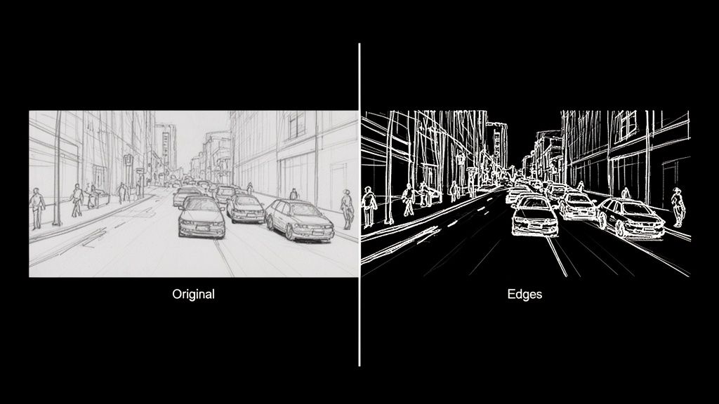
Imagine trying to describe a scene using only its outlines. That's precisely what a computer does with edge detection. It’s how machines begin to make sense of the visual chaos, much like an artist sketches the basic form of a subject before layering on color, shadow, and texture.

At its core, edge detection is a hunt for discontinuities. The goal is to scan a digital image and flag every point where the brightness of pixels changes abruptly. These sudden jumps are what we call "edges," and they almost always map directly to the boundaries of objects in the real world.

The Building Blocks of Machine Vision

Let’s get practical. An image is just a giant grid of numbers, with each number representing a pixel's brightness or color. An edge is simply where two neighboring numbers in that grid are wildly different. The sharp contrast between a dark t-shirt (low pixel value) and a white wall behind it (high pixel value) creates a perfect, high-contrast edge for an algorithm to find.

This simple idea is the bedrock of machine vision. As a fundamental tool in image processing, it's a key part of understanding what computer vision is and how it functions. Without first figuring out where a car stops and the road begins, higher-level tasks like tracking that car would be next to impossible.

This isn’t just some abstract theory; it's a powerful tool with massive real-world value. By turning a sea of pixels into a clean set of contours, you create a structural map that other, more complex algorithms can actually work with.

By dramatically cutting down the amount of data an algorithm has to sift through, edge detection lets computer vision systems zero in on an image's structural skeleton. This makes everything that comes next—like recognizing what the object actually is—way faster and more accurate.

From E-commerce to Autonomous Cars

Once you start looking, you'll see the applications are everywhere. E-commerce developers use it to slice product images out from their backgrounds for clean, professional-looking catalogs. In the auto industry, it’s absolutely critical for self-driving cars to spot lane markings, read road signs, and see other vehicles.

And it doesn't stop there. Other powerful use cases include:

• Medical Imaging: Radiologists and surgeons lean on edge detection to outline tumors, organs, and other structures in MRIs and X-rays.
• Augmented Reality (AR): AR apps need to find the edges of tables and walls to convincingly place virtual objects in your living room.
• Quality Control: On an assembly line, automated systems use it to spot tiny cracks, dents, or other defects on products zipping by.

For any developer, learning how to find these fundamental outlines is the first real step on the journey from basic theory to building some seriously impressive applications.

Meet The OGs: The Classic Edge Detection Algorithms

Long before deep learning became the star of the show, computer vision had its own set of grizzled, old-school detectives. These foundational algorithms were the original masters of deduction, designed to hunt down the most fundamental clue in any image: the edge. Let's pull back the curtain on the pioneers—the Sobel, Prewitt, and Roberts Cross operators.

Imagine an image isn't a picture, but a landscape. A solid block of color is a flat, grassy plain. An edge, where two different colors smash together, is a sheer cliff face. These classic algorithms act like digital surveyors, measuring the steepness—or gradient—of that cliff. A steeper drop-off means a sharper, more obvious edge.

Sobel: The Gradient Specialist

The Sobel operator is easily the most famous of the bunch, a true workhorse in the world of image processing. It works by sliding a tiny 3×3 window over every single pixel, calculating the gradient for both the horizontal and vertical directions. It’s basically asking two simple questions at every stop: "How much are things changing to my left and right?" and "How much are things changing above and below me?"

The clever part is that Sobel gives a little extra weight to the pixels closest to the center. This creates a subtle smoothing effect, which makes it much better at ignoring random image noise. That’s a massive plus when you're working with real-world photos, which are almost never perfectly clean.

This method was a game-changer back in the late 1960s. Introduced around 1968, the Sobel operator was one of the first truly effective ways to find boundaries by crunching the numbers on image intensity. A 2023 study focusing on industrial robotics even found that Sobel-based methods boosted the accuracy of object boundary detection by 25% over simpler techniques. You can dig into a brief history of these foundational models for a little more context.

Prewitt: The Unbiased Observer

The Prewitt operator is Sobel's no-nonsense cousin. It also uses a 3×3 kernel to check out a pixel's neighborhood and figure out the horizontal and vertical gradients. The big difference? Prewitt is all about equality—it gives the same importance to every surrounding pixel.

This democratic approach makes the Prewitt operator a tad faster to compute, but it also leaves it more vulnerable to noise. Think of it as the get-it-done-fast detective who might occasionally mistake a bit of static for a genuine lead.

• Core Idea: Approximates the image gradient, just like Sobel.
• Key Difference: Its kernels are unweighted, treating all neighboring pixels as equals.
• Result: It's computationally lighter but can be more easily fooled by random noise.

Roberts Cross: The Diagonal Scout

And then there's the Roberts Cross operator, the oldest and simplest of them all. Forget the 3×3 grid; Roberts Cross uses a tiny 2×2 window. This laser-focused view means it only cares about the diagonal differences between pixels.

Because its kernel is so small, Roberts Cross is lightning-fast but also the most likely to get tripped up by noise. It's fantastic at highlighting very fine, crisp edges, but any grain or imperfection in the image can throw it off, often resulting in thinner, weaker edge maps compared to its more robust counterparts.

Analogy in Action: Imagine these three are looking at a brick wall. Sobel would zero in on the strong horizontal and vertical mortar lines, seeing them clearly. Prewitt would also spot the mortar lines but might get a bit more distracted by the rough texture of the bricks themselves. Roberts Cross would be great at highlighting the sharp corners of each individual brick, but the bumpy surface of the brick faces could easily lead it astray.

Classic First-Order Edge Detector Comparison

So, which one should you pick? It really boils down to a classic trade-off: speed versus noise resistance. Sobel is usually the best all-rounder, but knowing the others gives you more tools in your belt.

This quick cheat sheet should help you decide which classic detective to call for your next case.

Operator	Core Concept	Best For	Key Weakness
Sobel	Weighted gradient calculation with a 3×3 kernel that emphasizes center pixels.	General edge detection where some noise resilience is needed. A great default choice.	Slightly more computationally intensive than Prewitt or Roberts Cross.
Prewitt	Unweighted gradient calculation with a 3×3 kernel that treats all neighbors equally.	Situations where speed is paramount and the image is relatively clean and noise-free.	More susceptible to noise due to the lack of pixel weighting or smoothing.
Roberts Cross	Diagonal difference calculation using a small 2×2 kernel.	Detecting very fine, high-frequency edges when computational cost must be minimal.	Highly sensitive to noise and tends to produce weaker edge responses.

These old-school methods really laid the groundwork for everything that came after. By understanding how they measure gradients, you start to build a real intuition for how computers begin to see and make sense of our visual world, one sharp change at a time.

A Deep Dive Into Advanced Edge Detection Techniques

While the classic operators like Sobel and Prewitt are great for a quick-and-dirty edge map, modern applications often need something with a lot more finesse. When you're after clean, continuous lines without all the noisy chatter, it's time to call in the heavyweights.

Let’s meet the two algorithms that really set the bar for quality: Canny and Marr-Hildreth.

The Canny Edge Detector: The Industry’s Gold Standard

Think of a master artist sketching a portrait. They don’t just start throwing dark lines on the canvas. They prepare the surface, lay down faint guidelines, carefully refine the contours, and then connect everything into a coherent whole. That's the exact philosophy behind the Canny edge detector, and it's why it’s widely considered the gold standard in the field.

Instead of a simple, one-shot calculation, the Canny algorithm is a sophisticated multi-step process. It's meticulously designed to hit three critical goals: find all the real edges, make sure those edges are razor-thin and precisely where they should be, and mark each one only once. This methodical approach is what makes it so darn effective.

John Canny's 1986 algorithm was a game-changer. It introduced a multi-stage process that was miles ahead in rejecting noise and pinpointing edges. Canny starts with a Gaussian smoothing step that can slash noise by up to 90% in messy images. Then, it follows up with gradient calculation, non-maximum suppression, and a clever dual-thresholding trick that locks in strong edges while linking them to weaker ones. Back in the '90s, benchmarks showed Canny outperforming Sobel by 40% in localization accuracy. It was a huge leap forward.

This flow diagram gives you a sense of how the classic methods work.

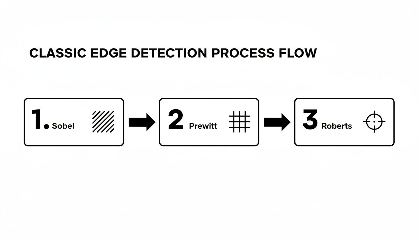
You can see how operators like Sobel and Prewitt are more of a direct, single-step affair, which really highlights the difference in complexity.

So, what’s the secret sauce? The Canny algorithm's magic lies in its four-stage pipeline:

1. Noise Reduction: It all starts with a Gaussian blur to smooth the image. This is a crucial first step because it gets rid of random pixel noise that could easily be mistaken for an edge, preventing a messy, cluttered output.
2. Gradient Calculation: Next, it uses a Sobel-like operator to figure out the direction and strength of intensity changes for every single pixel. This step essentially identifies all the potential edges.
3. Non-Maximum Suppression: This is where the real cleverness begins. It's a thinning process. The algorithm scans along the edge's direction and, if it finds a thick line of potential edge pixels, it keeps only the one with the strongest gradient. This is what gives you those beautiful, one-pixel-wide lines.
4. Hysteresis Thresholding: Finally, Canny uses two thresholds—one high, one low—to intelligently connect the dots. Any edge stronger than the high threshold is locked in as a "sure" edge. Any edge between the two thresholds is only kept if it’s connected to a "sure" edge. This brilliantly bridges gaps and creates clean, continuous outlines.

Marr-Hildreth: The Multi-Scale Detective

While Canny is all about creating that one perfect edge map, the Marr-Hildreth operator (also known as the Laplacian of Gaussian, or LoG) has a different trick up its sleeve. Think of it like a detective using different magnifying glasses to inspect a scene at various levels of detail.

The LoG operator first blurs the image with a Gaussian filter (just like Canny) and then applies a Laplacian operator to find the second derivative. The edges are found at the "zero-crossings"—the points where the output flips from positive to negative.

The real power here is scale. By using Gaussian filters of different sizes, the Marr-Hildreth method can spot edges at multiple scales.

• A large Gaussian filter smudges out the fine details, revealing only the big, bold outlines of major objects.
• A small Gaussian filter keeps things sharp, allowing it to pick up on fine textures and tiny boundaries.

This multi-scale perspective is invaluable. It lets an algorithm understand both the sweeping curve of a car's body and the crisp edge of its license plate at the same time, providing a much richer map of the image's structure.

These powerful contours are the building blocks for much more complex tasks. For example, high-quality boundaries are critical for things like segmentation in medical imaging, where you need to precisely isolate specific organs or tissues.

It’s the same story for high-end image manipulation. When you want to upscale an image, preserving those sharp edges is everything if you want to avoid a blurry, artificial-looking mess. You can see how modern AI handles this by checking out our image upscaling demo, where our models work hard to enhance images while keeping edges crisp. Moving beyond the classic methods is what lets us build the kind of robust and accurate vision systems that today’s applications demand.

Bringing Edge Detection to Life with Python and OpenCV

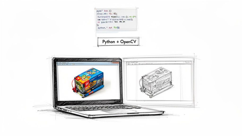
Alright, theory is one thing, but making those edges actually pop on your screen is where the real fun begins. Let's roll up our sleeves and turn those powerful concepts into working code using two of a developer's best friends: Python and the mighty OpenCV library.

OpenCV is a massive open-source computer vision library that makes implementing algorithms like Sobel and Canny feel almost like cheating. It handles all the heavy lifting—the nasty math, the pixel-by-pixel operations—so you can focus on getting fantastic results.

Implementing the Sobel Operator

Let's start with a classic: the Sobel operator. The goal here is simple—calculate the image's gradient to highlight where the pixel intensity changes most dramatically. With OpenCV, you can knock this out in just a few lines of code.

Here’s a basic recipe to get you started:

import cv2
import numpy as np

Load your image in grayscale

image = cv2.imread('your_image.jpg', cv2.IMREAD_GRAYSCALE)

Apply Sobel operator for X and Y directions

sobel_x = cv2.Sobel(image, cv2.CV_64F, 1, 0, ksize=3)
sobel_y = cv2.Sobel(image, cv2.CV_64F, 0, 1, ksize=3)

Combine the gradients to get the final edge map

sobel_combined = cv2.magnitude(sobel_x, sobel_y)

Convert back to a displayable format

sobel_combined = np.uint8(sobel_combined)

Display the result

cv2.imshow('Sobel Edges', sobel_combined)
cv2.waitKey(0)
cv2.destroyAllWindows()

In this little snippet, we calculate the horizontal (sobel_x) and vertical (sobel_y) gradients on their own first. Then we smash them together with cv2.magnitude to get a single, comprehensive map of all the edges, no matter which way they're pointing. It’s a super quick and effective way to get a first look at an image's structure.

Mastering the Canny Edge Detector

Now for the main event: the Canny algorithm. It's the industry go-to for a reason, delivering crisp, clean, and surprisingly intelligent edge maps. Its power comes from its multi-stage process, but the real magic for a developer lies in tuning its parameters.

The most crucial part is picking your two thresholds for the hysteresis step: threshold1 (the lower bound) and threshold2 (the upper bound).

Finding the right thresholds is more of an art than a science. Get them wrong, and you'll either have a canvas full of noisy, meaningless lines or an outline with frustrating gaps. Get them right, and you’ll produce a perfect, continuous contour.

Check out this starter code:

import cv2

Load your image in grayscale

image = cv2.imread('your_image.jpg', cv2.IMREAD_GRAYSCALE)

It's a good practice to blur the image first to reduce noise

blurred_image = cv2.GaussianBlur(image, (5,5), 0)

Apply the Canny edge detector

canny_edges = cv2.Canny(blurred_image, threshold1=100, threshold2=200)

Display the result

cv2.imshow('Canny Edges', canny_edges)
cv2.waitKey(0)
cv2.destroyAllWindows()

The Art of Tuning Canny Thresholds

So, how do you pick those magic numbers for threshold1 and threshold2? The results are incredibly sensitive to these values.

• If threshold2 is too low: The algorithm will think every bit of random noise is a "sure" edge, leaving you with a messy, cluttered output.
• If threshold1 is too high: The algorithm won't be brave enough to connect the weaker parts of a real edge, resulting in broken, disconnected lines.

A fantastic rule of thumb is to maintain a ratio between 1:2 or 1:3 for your lower and upper thresholds. For example, if you set threshold2 to 150, a good starting point for threshold1 would be 75 or 50. This simple guideline helps the algorithm effectively distinguish strong edges from noise while still connecting the dots along fainter contours.

Honestly, experimentation is key. Start with a baseline like (100, 200) and just start tweaking. See what happens. Every image is different, so what works for a clean product photo won't cut it for a busy landscape.

By mastering these simple implementations and learning how to feel out their parameters, you move from just running an algorithm to truly controlling it. For developers looking to integrate more advanced, edge-preserving functionalities directly into their applications, exploring a dedicated solution can be a great next step. You can see how these principles are applied in production-grade systems by checking out the PixelPanda API documentation, which offers powerful, pre-tuned models for tasks like background removal and smart enhancement. This hands-on experience is what transforms theoretical knowledge of edge detection in image processing into a practical, powerful skill.

The Future of Edge Detection with AI and Deep Learning

You could say the classic algorithms walked so that modern AI could run. Techniques like Sobel and Canny are the bedrock of computer vision, but the real magic in edge detection in image processing today comes from deep learning. This is where we stop telling the machine how to find edges with math and start teaching it to see them like we do.

Let's be honest, traditional algorithms can be a bit clumsy. They see a sudden change in pixel brightness and shout, "Edge!" But is that a real object boundary, or just the busy texture on a knitted sweater? They can't always tell the difference, which often leads to messy, noisy outlines. AI models, on the other hand, are trained on millions of images. They learn the subtle difference between a meaningful contour and distracting surface noise.

Beyond Pixels to Seeing the Bigger Picture

Deep learning, especially with Convolutional Neural Networks (CNNs), completely flips the script. Instead of just squinting at a pixel's immediate neighbors, these networks learn to understand the entire object's context. A well-trained model knows what a person's silhouette is supposed to look like, letting it draw a clean line around them while completely ignoring the pattern on their shirt.

This isn't an overnight breakthrough; it's a leap built on decades of research. The Marr-Hildreth detector, developed back in the late 1970s, introduced the Laplacian of Gaussian (LoG) operator. This idea of smoothing an image before looking for edges paved the way for later innovations. It influenced everything from SIFT algorithms to the deep learning explosion kicked off by models like AlexNet in 2012, which radically cut down image recognition errors. The foundational ideas are still with us.

Today, that rich history is what powers platforms like PixelPanda. We've taken those core concepts and supercharged them to do things like depth-aware upscaling, which keeps edges unbelievably sharp. It’s the difference between a simple line drawing and a genuine understanding of an object's shape.

AI models don't just find edges; they find the right edges. By learning from vast datasets, they can infer the complete boundary of an object even when parts of it are obscured or have low contrast—a task that leaves traditional methods struggling.

Putting AI in Your Hands with APIs

Let's face it: training and deploying these sophisticated models is a massive undertaking. It’s a huge barrier for most developers. That’s where a good API comes in, doing all the machine learning heavy lifting for you. You don’t need a Ph.D. in computer vision anymore; you just need to make an API call to get incredible results.

This approach gives developers an almost unfair advantage. Think about background removal—a notoriously painful task, especially with tricky details like hair or fur. An AI-powered tool can create cutouts that preserve individual strands of hair, a level of detail that’s practically impossible to get right with classic edge detection alone.

• Precision: AI uses semantic understanding to tell the difference between a person and the wall behind them.
• Efficiency: It turns a tedious, hours-long manual editing job into an automated, split-second process.
• Scalability: It lets you process thousands of images with perfect consistency, day in and day out.

The bottom line is this: knowing the classic algorithms gives you a fantastic foundation. But if you want the jaw-dropping quality and automation that today's apps demand, AI is the only way to go. You can see this for yourself by playing with our background removal demo, which shows just how gracefully these advanced models handle even the most complex edges. This is the future—not just finding lines, but truly understanding them.

A Few Common Edge Detection Head-Scratchers

Jumping into edge detection can feel a bit like learning to cook a new dish. You follow the recipe (the algorithm), but then you hit those little snags that only experience can solve. This section is for those moments—a quick FAQ to tackle the real-world problems that pop up when you're in the weeds.

Which Algorithm Should I Use for Real-Time Video?

When you’re working with video, every millisecond counts. Speed is the name of the game. For raw, blistering speed, simple operators like Sobel are often your best bet. They're incredibly lightweight and get the job done without a lot of computational fuss.

But don't write off Canny just yet. While it’s definitely the more resource-hungry of the two, modern hardware and optimized libraries like OpenCV can make it surprisingly zippy. A well-tuned Canny implementation can often keep up with many video streams. My advice? Benchmark both on the actual hardware you'll be using. Start with Sobel if you need every last drop of performance, but if the edge quality isn't quite there, see if you have the headroom to switch to Canny.

How Do I Deal With Noisy Images Before Finding Edges?

Noise is the sworn enemy of good edge detection. It's the static that creates fake edges, shatters clean lines, and generally makes a mess of your results. Your first line of defense, and your best friend here, is a Gaussian blur.

You absolutely have to apply a blur before running your edge detector. In fact, it's so crucial that it’s baked right into the Canny algorithm as the very first step. The size of the blur kernel you pick (like a 3×3 or 5×5 grid) controls how much smoothing you apply.

• A larger kernel smooths things out aggressively, which is great for heavy noise but can also obliterate fine details.
• A smaller kernel is much more gentle, preserving those delicate edges but potentially leaving some noise behind.

Quick tip: if your image is covered in "salt-and-pepper" noise (those random black and white specks), a Median filter can sometimes work miracles where a Gaussian blur falls short.

It’s all a balancing act. You're trying to quiet the noise just enough without smudging the actual edges you care about. I always start with a small kernel and slowly dial it up until I hit that sweet spot.

Why Are My Canny Edges Broken or Full of Static?

Ah, the classic Canny problem. If you’re seeing this, I’d bet my lunch money the issue is with your two threshold values: minVal and maxVal. If your image is a chaotic mess of tiny, staticky lines, your high threshold is set too low. The algorithm is getting confused and thinking every little bit of noise is a "strong" edge.

On the flip side, if your edges are clean but have frustrating gaps in them, your low threshold is probably too high. This stops the algorithm from connecting the weaker parts of a real edge back to the stronger parts it already found. A great rule of thumb that works surprisingly often is the 1:2 or 1:3 ratio. First, find a maxVal that only picks up the most obvious, strongest edges. Then, set your minVal to half or even a third of that value. This gives the algorithm enough leeway to intelligently trace the rest of the line.

---

For those really tough cases—think wispy hair, delicate fur, or intricate product details—sometimes a traditional algorithm just won't cut it. That's where AI-powered tools like PixelPanda come in. Our models understand the content of an image, not just the math of pixel gradients, giving you stunningly accurate results. See how our edge-preserving API can transform your visual workflow at https://pixelpanda.ai.